Understanding LMS-based Color Blindness Simulations
Diving deeper in the theory of Viénot, Brettel & Mollon's method to understand what's behind the scene.


- Introduction
- From sRGB to LMS
- Simulating dichromacy in LMS (Brettel 1997 and Viénot 1999)
- Comparing Viénot 1999 and Brettel 1997
- What about anomalous trichromacy?
- Conclusion
- Bibliography
- Appendix
Introduction
This post is a followup to our Review of Open Source Color Blindness Simulations and assumes that you are familiar with color vision deficiencies (CVD) simulation. The goal of this post is to dive into how these methods actually work. To visualize and play with the models interactively this page is actually generated from a Jupyter notebook (using fastpages) and can be run in e.g. Google colab to play with it.
The interactive 3D plots make it hard to read on mobile, a large screen is recommended.
(Brettel, Viénot, & Mollon, 1997), (Viénot, Brettel, & Mollon, 1999) and (Machado, Oliveira, & Fernandes, 2009) all rely on the same low-level principles to simulate CVD. For all of them the final code will basically just apply a sRGB/gamma function, one or two 3x3 matrices, undo the gamma, and call it a day. But we're going to analyze that pipeline and try to understand how to compute those matrices and get a sense of what they do.
The Machado 2009 method is actually a bit more involved as it uses a second stage of modeling (opponent-color theory), so we will not cover it here and only focus on Viénot 1999 and Brettel 1997. Both focus on full dichromacy, so we'll start with that. It's worth noting that Machado 2009 has similar results for dichromacy anyway, and the extension to anomalous trichromacy will be discussed in section What about anomalous trichromacy?.
Let's first get an overview of the process. Protanopes, deuteranopes and tritanopes respectively lack the L, M, and S cone cells. Thus a natural approach to simulate dichromacy is to go to the LMS color-space and somehow remove the component coming from the missing cone cells. The good news is that going from an RGB color space to LMS can be done with a linear transformation (matrix multiplication). But as usual there are many ways to do it and it'll deserve its own section.
One extra complexity is that images are typically encoded in sRGB to get properly displayed on digital monitors. So our first step will be to go from sRGB to linear RGB, and then from there to LMS.
Once in the LMS color space, colors that only differ by the coordinate of the axis corresponding to the missing cone cannot be differentiated by a dichromat. This creates so-called confusion lines, which are, by construction, parallel to the missing axis in the LMS color space. So according to this model a protanope cannot distinguish colors that only differ by their L component, a deuteranope those that only differ by their M component, and tritanopes those that only differ by their S component.
To illustrate this let's build a plot with a few confusion lines in the LMS space, and their counterpart on the linear RGB space. The code to generate the confusion lines is in the Appendix. We're going to just draw 5 precomputed lines, starting with protanopia (missing L cones). To have a reference we'll also add the gamut (range) of colors that can be produced by a digital monitor. It's a cube in the RGB color space, and a parallelepiped in the LMS space. The 8 vertices are black (K = RGB[0,0,0]), white (W = RGB[1, 1, 1]), red (R = RGB[1, 0, 0]), green (G = RGB[0,1,0]), blue (B = RGB[0,0,1]), yellow (Y = RGB[1,1,0]), magenta (M = RGB[1,0,1]) and cyan (C = RGB[0,1,1]).
The plots are in 3D and interactive, so feel free to play with the point of view!
# This cell defines all our imports and a few utilities
import itertools
import numpy as np
import plotly.express as px
import plotly.graph_objs as go
from plotly.subplots import make_subplots
import pandas as pd
import Geometry3D as geo3d

import daltonlens.convert as convert
import daltonlens.generate as generate
import daltonlens.simulate as simulate
import daltonlens.geometry as geometry
np.set_printoptions(suppress=True)

def printMatrix(name, m):
    mat_str = '\n  '.join(np.array_repr(m).split('\n'))
    print (f'{name} = \n  {mat_str}')

# Utility for plotly imshow
hide_image_axes = dict(yaxis_visible=False, yaxis_showticklabels=False, xaxis_visible=False, xaxis_showticklabels=False, margin=dict(l=0, r=0, b=0, t=0))
def show_confusion_lines(title, lines):
    rgb_cube = pd.DataFrame.from_records([
        ('K', 'black',     0,   0,   0, 0.        , 0.        , 0.        , '#000000'),
        ('B', 'blue',      0,   0,   1, 0.03596577, 0.03620635, 0.01528089, '#0000ff'),
        ('M', 'magenta',   1,   0,   1, 0.21482533, 0.07001029, 0.01559176, '#ff00ff'),
        ('R', 'red',       1,   0,   0, 0.17885956, 0.03380394, 0.00031087, '#ff0000'),
        ('G', 'green',     0,   1,   0, 0.43997117, 0.27515242, 0.00191661, '#00ff00'),
        ('C', 'cyan',      0,   1,   1, 0.47593694, 0.31135877, 0.0171975 , '#00ffff'),
        ('W', 'white',     1,   1,   1, 0.6547965 , 0.34516271, 0.01750837, '#ffffff'),
        ('Y', 'yellow',    1,   1,   0, 0.61883073, 0.30895636, 0.00222748, '#ffff00')],
        columns = ['short_name', 'name', 'R', 'G', 'B', 'L', 'M', 'S', 'sRGB_hex'])
    rgb_cube.index = rgb_cube['short_name']
    rgb_cube.index.name = 'key'
    # display(HTML("<h2>RGB Cube</h2>"), rgb_cube)

    fig = make_subplots(1,2,
                        subplot_titles=('RGB Color Space',  'LMS Color Space'),
                        specs=[[{"type": "scene"}, {"type": "scene"}]])

    fig.add_scatter3d(x=rgb_cube['R'], y=rgb_cube['G'], z=rgb_cube['B'],
                      text=rgb_cube.index, mode="markers+text",
                      showlegend=False,
                      marker=dict(color=rgb_cube['sRGB_hex']),
                      row=1, col=1)

    fig.add_scatter3d(x=rgb_cube['L'], y=rgb_cube['M'], z=rgb_cube['S'],
                      text=rgb_cube.index, mode="markers+text",
                      showlegend=False,
                      marker=dict(color=rgb_cube['sRGB_hex']),
                      row=1, col=2)

    fig.update_layout(title=title)

    fig.update_layout(dragmode='orbit',
                      scene = dict(
                        xaxis_title='R',
                        yaxis_title='G',
                        zaxis_title='B'))

    fig.update_layout(scene2 = dict(
                        xaxis_title='L',
                        yaxis_title='M',
                        zaxis_title='S'))

    # Add the parallelepiped lines
    df = rgb_cube.loc[['K','B','M','R', 'K', 'G', 'Y', 'W', 'C', 'G', 'Y', 'R', 'M', 'W', 'C', 'B']]
    fig.add_scatter3d(x=df['R'], y=df['G'], z=df['B'], mode='lines', showlegend=False, row=1, col=1)
    fig.add_scatter3d(x=df['L'], y=df['M'], z=df['S'], mode='lines', showlegend=False, row=1, col=2)

    for line in lines:
        fig.add_scatter3d(x=line['R'], y=line['G'], z=line['B'], showlegend=False,
                          marker=dict(color=line['sRGB_hex']),
                          row=1, col=1)

        fig.add_scatter3d(x=line['L'], y=line['M'], z=line['S'], showlegend=False,
                          marker=dict(color=line['sRGB_hex']),
                          row=1, col=2)

    fig.show()

# Confusion lines for Deficiency.PROTAN
protan_confusion_lines = [
    pd.DataFrame.from_records([
        (0.2299, 0.0690, 0.0034, 1.0000, 0.0987, 0.1964, '#fe587a'),
        (0.2093, 0.0690, 0.0034, 0.8333, 0.1198, 0.1971, '#eb617a'),
        (0.1887, 0.0690, 0.0034, 0.6667, 0.1409, 0.1979, '#d5687a'),
        (0.1681, 0.0690, 0.0034, 0.5000, 0.1620, 0.1986, '#bb6f7b'),
        (0.1475, 0.0690, 0.0034, 0.3334, 0.1831, 0.1994, '#9c767b'),
        (0.1269, 0.0690, 0.0034, 0.1667, 0.2042, 0.2002, '#717c7b'),
        (0.1063, 0.0690, 0.0034, 0.0001, 0.2253, 0.2009, '#00827b')],
        columns = ['L', 'M', 'S', 'R', 'G', 'B', 'sRGB_hex']),
    pd.DataFrame.from_records([
        (0.2658, 0.1724, 0.0084, 0.0000, 0.5633, 0.5023, '#00c5bb'),
        (0.2864, 0.1724, 0.0084, 0.1667, 0.5422, 0.5015, '#71c2bb'),
        (0.3070, 0.1724, 0.0084, 0.3333, 0.5211, 0.5008, '#9cbfbb'),
        (0.3276, 0.1724, 0.0084, 0.5000, 0.5000, 0.5000, '#bbbbbb'),
        (0.3482, 0.1724, 0.0084, 0.6666, 0.4789, 0.4992, '#d5b7bb'),
        (0.3688, 0.1724, 0.0084, 0.8333, 0.4578, 0.4985, '#ebb4bb'),
        (0.3894, 0.1724, 0.0084, 0.9999, 0.4367, 0.4977, '#feb0bb')],
        columns = ['L', 'M', 'S', 'R', 'G', 'B', 'sRGB_hex']),
    pd.DataFrame.from_records([
        (0.2770, 0.1055, 0.0115, 1.0000, 0.1550, 0.7466, '#fe6de0'),
        (0.2565, 0.1055, 0.0115, 0.8333, 0.1761, 0.7474, '#eb74e0'),
        (0.2359, 0.1055, 0.0115, 0.6667, 0.1972, 0.7481, '#d57ae0'),
        (0.2153, 0.1055, 0.0115, 0.5000, 0.2183, 0.7489, '#bb80e0'),
        (0.1947, 0.1055, 0.0115, 0.3334, 0.2394, 0.7496, '#9c86e0'),
        (0.1741, 0.1055, 0.0115, 0.1667, 0.2605, 0.7504, '#718be0'),
        (0.1535, 0.1055, 0.0115, 0.0001, 0.2816, 0.7511, '#0090e0')],
        columns = ['L', 'M', 'S', 'R', 'G', 'B', 'sRGB_hex']),
    pd.DataFrame.from_records([
        (0.5017, 0.2393, 0.0053, 1.0000, 0.7183, 0.2489, '#fedc88'),
        (0.4811, 0.2393, 0.0053, 0.8333, 0.7394, 0.2496, '#ebdf88'),
        (0.4605, 0.2393, 0.0053, 0.6667, 0.7605, 0.2504, '#d5e289'),
        (0.4399, 0.2393, 0.0053, 0.5000, 0.7816, 0.2511, '#bbe489'),
        (0.4193, 0.2393, 0.0053, 0.3334, 0.8027, 0.2519, '#9ce789'),
        (0.3987, 0.2393, 0.0053, 0.1667, 0.8239, 0.2526, '#71ea89'),
        (0.3781, 0.2393, 0.0053, 0.0001, 0.8450, 0.2534, '#00ec89')],
        columns = ['L', 'M', 'S', 'R', 'G', 'B', 'sRGB_hex']),
    pd.DataFrame.from_records([
        (0.4253, 0.2758, 0.0135, 0.0000, 0.9013, 0.8036, '#00f3e7'),
        (0.4459, 0.2758, 0.0135, 0.1667, 0.8802, 0.8029, '#71f1e7'),
        (0.4665, 0.2758, 0.0135, 0.3333, 0.8591, 0.8021, '#9ceee7'),
        (0.4871, 0.2758, 0.0135, 0.5000, 0.8380, 0.8014, '#bbebe7'),
        (0.5077, 0.2758, 0.0135, 0.6666, 0.8169, 0.8006, '#d5e9e7'),
        (0.5283, 0.2758, 0.0135, 0.8333, 0.7958, 0.7998, '#ebe6e7'),
        (0.5488, 0.2758, 0.0135, 0.9999, 0.7747, 0.7991, '#fee3e6')],
        columns = ['L', 'M', 'S', 'R', 'G', 'B', 'sRGB_hex']),
]

show_confusion_lines('Examples of protan confusion lines', protan_confusion_lines)
The colors of some of the 5 lines might be easier to discriminate for some protan, but overall with this point size they should be pretty difficult to differentiate on a monitor screen.
See how the confusion lines are parallel to the L axis in the LMS color space, but not aligned with any axis in the RGB space. As expected for protanopes, the colors along the confusion lines vary mostly by their red and green components and are pretty much orthogonal to the blue axis.
Let's also visualize some lines for deuteranopes (parallel to the M axis) and tritanopes (parallel to the S axis).
# Confusion lines for Deficiency.DEUTAN
deutan_confusion_lines = [
    pd.DataFrame.from_records([
        (0.1310, 0.0843, 0.0034, 0.0000, 0.2828, 0.1937, '#009079'),
        (0.1310, 0.0756, 0.0034, 0.1139, 0.2357, 0.1973, '#5e857a'),
        (0.1310, 0.0668, 0.0034, 0.2277, 0.1885, 0.2009, '#83787b'),
        (0.1310, 0.0581, 0.0034, 0.3416, 0.1414, 0.2045, '#9d697c'),
        (0.1310, 0.0494, 0.0034, 0.4554, 0.0943, 0.2081, '#b3567d'),
        (0.1310, 0.0407, 0.0034, 0.5693, 0.0471, 0.2117, '#c63d7e'),
        (0.1310, 0.0319, 0.0034, 0.6831, 0.0000, 0.2153, '#d7007f')],
        columns = ['L', 'M', 'S', 'R', 'G', 'B', 'sRGB_hex']),
    pd.DataFrame.from_records([
        (0.3276, 0.1341, 0.0084, 1.0000, 0.2930, 0.5158, '#fe93be'),
        (0.3276, 0.1468, 0.0084, 0.8333, 0.3620, 0.5105, '#eba2bd'),
        (0.3276, 0.1596, 0.0084, 0.6667, 0.4310, 0.5053, '#d5afbc'),
        (0.3276, 0.1724, 0.0084, 0.5000, 0.5000, 0.5000, '#bbbbbb'),
        (0.3276, 0.1852, 0.0084, 0.3334, 0.5690, 0.4947, '#9cc6ba'),
        (0.3276, 0.1979, 0.0084, 0.1667, 0.6380, 0.4895, '#71d1b9'),
        (0.3276, 0.2107, 0.0084, 0.0001, 0.7069, 0.4842, '#00dab8')],
        columns = ['L', 'M', 'S', 'R', 'G', 'B', 'sRGB_hex']),
    pd.DataFrame.from_records([
        (0.1844, 0.1247, 0.0115, 0.0000, 0.3535, 0.7421, '#00a0df'),
        (0.1844, 0.1138, 0.0115, 0.1423, 0.2946, 0.7466, '#6993e0'),
        (0.1844, 0.1029, 0.0115, 0.2846, 0.2357, 0.7511, '#9185e0'),
        (0.1844, 0.0920, 0.0115, 0.4270, 0.1768, 0.7556, '#ae74e1'),
        (0.1844, 0.0811, 0.0115, 0.5693, 0.1178, 0.7601, '#c660e1'),
        (0.1844, 0.0702, 0.0115, 0.7116, 0.0589, 0.7646, '#db44e2'),
        (0.1844, 0.0593, 0.0115, 0.8539, 0.0000, 0.7691, '#ed00e3')],
        columns = ['L', 'M', 'S', 'R', 'G', 'B', 'sRGB_hex']),
    pd.DataFrame.from_records([
        (0.4708, 0.2201, 0.0053, 1.0000, 0.6465, 0.2579, '#fed28a'),
        (0.4708, 0.2310, 0.0053, 0.8577, 0.7054, 0.2534, '#eeda89'),
        (0.4708, 0.2419, 0.0053, 0.7154, 0.7643, 0.2489, '#dbe288'),
        (0.4708, 0.2528, 0.0053, 0.5730, 0.8232, 0.2444, '#c7ea87'),
        (0.4708, 0.2637, 0.0053, 0.4307, 0.8822, 0.2399, '#aff186'),
        (0.4708, 0.2746, 0.0053, 0.2884, 0.9411, 0.2354, '#92f885'),
        (0.4708, 0.2855, 0.0053, 0.1461, 1.0000, 0.2309, '#6afe84')],
        columns = ['L', 'M', 'S', 'R', 'G', 'B', 'sRGB_hex']),
    pd.DataFrame.from_records([
        (0.5241, 0.3128, 0.0135, 0.3168, 1.0000, 0.7847, '#98fee5'),
        (0.5241, 0.3041, 0.0135, 0.4307, 0.9529, 0.7883, '#aff9e5'),
        (0.5241, 0.2954, 0.0135, 0.5445, 0.9057, 0.7919, '#c2f4e6'),
        (0.5241, 0.2867, 0.0135, 0.6584, 0.8586, 0.7955, '#d4eee6'),
        (0.5241, 0.2780, 0.0135, 0.7722, 0.8115, 0.7991, '#e3e8e7'),
        (0.5241, 0.2692, 0.0135, 0.8861, 0.7644, 0.8027, '#f1e2e7'),
        (0.5241, 0.2605, 0.0135, 1.0000, 0.7172, 0.8063, '#fedce7')],
        columns = ['L', 'M', 'S', 'R', 'G', 'B', 'sRGB_hex']),
]

show_confusion_lines('Examples of deutan confusion lines', deutan_confusion_lines)
# Confusion lines for Deficiency.TRITAN
tritan_confusion_lines = [
    pd.DataFrame.from_records([
        (0.1310, 0.0690, 0.0005, 0.1663, 0.2328, 0.0000, '#718400'),
        (0.1310, 0.0690, 0.0029, 0.1944, 0.2055, 0.1667, '#797d71'),
        (0.1310, 0.0690, 0.0053, 0.2224, 0.1782, 0.3333, '#81759c'),
        (0.1310, 0.0690, 0.0077, 0.2505, 0.1509, 0.5000, '#896cbb'),
        (0.1310, 0.0690, 0.0101, 0.2785, 0.1236, 0.6666, '#8f62d5'),
        (0.1310, 0.0690, 0.0125, 0.3066, 0.0963, 0.8333, '#9657eb'),
        (0.1310, 0.0690, 0.0149, 0.3346, 0.0689, 0.9999, '#9c4afe')],
        columns = ['L', 'M', 'S', 'R', 'G', 'B', 'sRGB_hex']),
    pd.DataFrame.from_records([
        (0.3276, 0.1724, 0.0156, 0.5842, 0.4181, 1.0000, '#c9adfe'),
        (0.3276, 0.1724, 0.0132, 0.5561, 0.4454, 0.8333, '#c4b2eb'),
        (0.3276, 0.1724, 0.0108, 0.5281, 0.4727, 0.6667, '#c0b6d5'),
        (0.3276, 0.1724, 0.0084, 0.5000, 0.5000, 0.5000, '#bbbbbb'),
        (0.3276, 0.1724, 0.0060, 0.4720, 0.5273, 0.3334, '#b6c09c'),
        (0.3276, 0.1724, 0.0036, 0.4439, 0.5546, 0.1667, '#b1c471'),
        (0.3276, 0.1724, 0.0012, 0.4159, 0.5819, 0.0001, '#acc800')],
        columns = ['L', 'M', 'S', 'R', 'G', 'B', 'sRGB_hex']),
    pd.DataFrame.from_records([
        (0.1844, 0.1055, 0.0007, 0.1238, 0.3729, 0.0000, '#62a400'),
        (0.1844, 0.1055, 0.0031, 0.1518, 0.3456, 0.1667, '#6c9e71'),
        (0.1844, 0.1055, 0.0055, 0.1799, 0.3183, 0.3333, '#75989c'),
        (0.1844, 0.1055, 0.0079, 0.2079, 0.2910, 0.5000, '#7d92bb'),
        (0.1844, 0.1055, 0.0103, 0.2360, 0.2637, 0.6666, '#858cd5'),
        (0.1844, 0.1055, 0.0127, 0.2640, 0.2364, 0.8333, '#8c85eb'),
        (0.1844, 0.1055, 0.0151, 0.2921, 0.2091, 0.9999, '#937efe')],
        columns = ['L', 'M', 'S', 'R', 'G', 'B', 'sRGB_hex']),
    pd.DataFrame.from_records([
        (0.4708, 0.2393, 0.0161, 0.8762, 0.6271, 1.0000, '#f0cffe'),
        (0.4708, 0.2393, 0.0137, 0.8482, 0.6544, 0.8333, '#edd3eb'),
        (0.4708, 0.2393, 0.0113, 0.8201, 0.6817, 0.6667, '#e9d7d5'),
        (0.4708, 0.2393, 0.0089, 0.7921, 0.7090, 0.5000, '#e6dbbb'),
        (0.4708, 0.2393, 0.0065, 0.7640, 0.7363, 0.3334, '#e2de9c'),
        (0.4708, 0.2393, 0.0041, 0.7360, 0.7636, 0.1667, '#dee271'),
        (0.4708, 0.2393, 0.0017, 0.7079, 0.7909, 0.0001, '#dae500')],
        columns = ['L', 'M', 'S', 'R', 'G', 'B', 'sRGB_hex']),
    pd.DataFrame.from_records([
        (0.5241, 0.2758, 0.0019, 0.6654, 0.9311, 0.0000, '#d4f700'),
        (0.5241, 0.2758, 0.0043, 0.6934, 0.9038, 0.1667, '#d8f371'),
        (0.5241, 0.2758, 0.0067, 0.7215, 0.8765, 0.3333, '#dcf09c'),
        (0.5241, 0.2758, 0.0091, 0.7495, 0.8492, 0.5000, '#e0edbb'),
        (0.5241, 0.2758, 0.0115, 0.7776, 0.8218, 0.6666, '#e4e9d5'),
        (0.5241, 0.2758, 0.0139, 0.8056, 0.7945, 0.8333, '#e7e6eb'),
        (0.5241, 0.2758, 0.0163, 0.8337, 0.7672, 0.9999, '#ebe2fe')],
        columns = ['L', 'M', 'S', 'R', 'G', 'B', 'sRGB_hex']),
]

show_confusion_lines('Examples of tritan confusion lines', tritan_confusion_lines)
The deutan confusion lines are somewhat similar to the protan confusion lines (this is why both are called red-green deficiency), but the tritan ones are mostly along the blue axis.
At this stage if you are affected by a color vision deficiency you might already have a more precise idea of what kind of dichromacy better models your color vision. For me the colors on the protan confusion lines look pretty similar at such a small point size, but I can better distinguish the deutan lines and very well the tritan ones, confirming that I am a protan.
Dichromats confusion lines are sometimes shown in the CIE XYZ color space (e.g. on color-blindness.com), usually drawing the lines on a so-called chromaticity diagram. These diagram are a 2d projection of the CIE XYZ color space for a constant maximal luminance. I always got confused about those because I could clearly see differences along these lines, especially when they transition from green to red. The reason is that the confusion lines are actually 3d in CIE XYZ and the luminance needs to get adjusted as the hue/chroma changes along the line to actually get confused by a dichromat. So now that we can compute these confusion lines for each kind of dichromacy, can we simulate how a person with a CVD sees? Since it's related to perception it's impossible to know how another person "feels" the colors, but to understand the loss of color sensitivity we can transform images so that all the colors on each confusion line projects to a single one, essentially making the color space 2D. If the models are correct then the transformed image should still appear identical to a dichromat, and a trichromat will get a sense of the color differences that get lost for the dichromat.
The remaining question is what color should we pick to represent each confusion line? That will be the subject of the Simulating dichromacy in LMS) section.
Finally once the LMS colors are projected along the confusion lines, we can transform them back to the linearRGB and then sRGB color spaces to get the final simulated image. The overall process is summarized in the diagram below, and we're going to dive into each part in the next sections.

From sRGB to LMS
In this section we're going to review the steps to go to that nice LMS color space. Several models have been proposed in the literature, so there is not just one way to do it.
From sRGB to linearRGB
Most digital images are encoded with 3 values per pixel: red, green and blue. But what is often neglected is that this "RGB" usually corresponds to the sRGB standard that precisely defines how these values should be interpreted. sRGB is not a linear space because it tries to compensate the non-linear gamma factor applied by monitors, so that the image captured by a digital camera and then rendered on a monitor will look like the original scene.
We'll call the RGB color space after removing that non-linearity the linearRGB color space. The transformation roughly corresponds to applying a gamma exponent of 2.4 on each channel, with a special linear slope for small values. So unlike all the other color transformations of that notebook it is non-linear and cannot be expressed as a matrix.
The good news is that sRGB is a well-defined standard now, so we just need to implement the function given by the standard. For more details see the wikipedia page.
Since both Brettel 1997 and Viénot 1999 were published before the sRGB standard became mainstream, they use a different model in their paper. Brettel 1997 calibrated a CRT monitor with a spectroradiometer to estime the spectral distribution of the primaries, while Viénot used a constant gamma of 2.2 to convert to linearRGB. Fortunately once in that space it uses the same BT.709 chromaticities as the sRGB standard, so it does not need to be adapted. However it's worth noting that even if the Viénot 1999 paper explicitly mentions the required non-linear gamma transform for their CRT monitor, the most widely replicated matlab code from (Fidaner, Lin, & Ozguven, 2005) does not take it into account and directly treat the input image as linear RGB. As a consequence this is also the case of most of the source code listed on websites like daltonize.org.
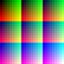
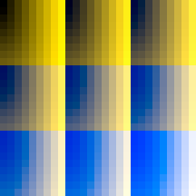
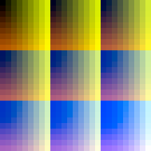
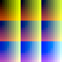
im_sRGB = np.array([[[127,0,0], [64,128,0], [0, 0, 192], [64, 64, 192]]], dtype=float) / 255.0
px.imshow(np.vstack([im_sRGB, # First row is the sRGB content
                     convert.linearRGB_from_sRGB(im_sRGB)]), height=200).update_layout(hide_image_axes)
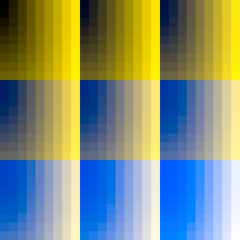
And the impact is also significant on the final simulation, here is a comparison of Viénot 1999 implemented with and without the proper sRGB decoding / encoding. Note how a bunch of colors appear too dark in the simulation without sRGB.
| Original | Viénot 1999 | Viénot 1999 without sRGB |
|---|---|---|
|
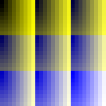
|
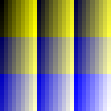
|
From linearRGB to CIE XYZ
So far we only mentioned the LMS color space, saying that we'd just go from linearRGB to LMS. But to understand the literature around that transform it is necessary to add an intermediate step which is the CIE XYZ color space. The reason is historical, this color space was standardized in 1931 and it has been used as the main space for color science research since. The main reason is that it can (almost) represent the full range of colors that can be perceived by an average human observer with just 3 values, is device-independent, and has a well-defined relationship w.r.t the input light spectrum.
The sRGB wikipedia page gives the XYZ_from_linearRGB matrix defined by the standard itself. But we need to be careful, as this assumes the CIE XYZ 1931 color space. Some LMS_from_XYZ transforms might assume a different XYZ color space. For example, as noted in Viénot 1999, the LMS from XYZ transform given by (Smith & Pokorny, 1975) is defined on top of the Judd-Vos corrected XYZ space. As another example the (Stockman & Sharpe, 2000) one assumes the XYZ space from the Stiles and Burch 10-deg CMFs adjusted to 2-deg.
This section was initially wrong and got updated in December 2021. Before I was assuming that Viénot 1999 was using an outdated model for CRT monitors and I ignored the Judd-Vos correction. But only the non-linear gamma was outdated, the XYZ from linearRGB was using the same BT.709 standard, so that conversion is still valid. Many thanks to Paul Maximov who pointed this out and helped me understand that part.
It's easy to get this wrong, but eventually Viénot proposed a pretty good approximation with a single XYZJuddVos_from_linearRGB matrix, which can then get combined with the LMS_from_RGB by Smith & Pokorny. They evaluated their approximation properly, so refer to the paper for the full details.
printMatrix('sRGB XYZJuddVos_from_linearRGB', convert.LMSModel_sRGB_SmithPokorny75().XYZ_from_linearRGB*100)
From CIE XYZ to LMS
That conversion is less clear as many more transforms have been proposed, with different motivations, and even different source XYZ color spaces as we've just seen.
The reference conversion for CVD simulation is probably still (Smith & Pokorny, 1975), which is the one used by (Viénot, Brettel, & Mollon, 1999). The earlier seminal work of (Meyer & Greenberg, 1988) used another transform from (Estévez, 1981) but it already mentioned (Smith & Pokorny, 1975) as being a good candidate. Another popular reference model in the literature is the Hunt-Pointer-Esterez one (Hunt, 2004). It is used a lot for chromatic adaptation (predicting how a perceived color will change with the illumination conditions), but less for CVD simulation experiments.
(Stockman & Sharpe, 2000) made a thorough comparison of the models, and they also propose a new matrix (for a 10 degree standard observer). But overall they are in good agreement with (Smith & Pokorny, 1975) once adjusted for a 2 degree observer, with larger differences compared to Hunt-Pointer-Esterez. All 3 are probably reasonable options, but since the CVD simulation evaluations were most often made and evaluated with Smith & Pokorny it's probably still the most solid choice, despite its age. It is also interesting to note that both Pokorny and Viénot continued to promote that transform in more recent papers (Viénot & Le Rohellec, 2013) (Smith & Pokorny, 2003), and other recent papers in the color science research literature do the same (Machado, Oliveira, & Fernandes, 2009) (Simon-Liedtke & Farup, 2016).
Most open source code also uses the Smith and Pokorny since they did not modify the original code, but some did. Ixora.io uses the Hunt-Pointer-Estevez matrix and daltonize.py uses the sharpened transformation matrix of CIECAM02. These two matrices are on the LMS Wikipedia page and look attractive as they are more recent. But at least the "sharpened" matrices variants were not designed to match the physiological cone responses but to perform hue-preserving chromatic adaptation (see the discussion p181 of (Fairchild, 2013)). The wikipedia page also says A "spectually sharpened" matrix is believed to improve chromatic adaptation especially for blue colors, but does not work as a real cone-describing LMS space for later human vision processing. So I would argue that we should keep using the Smith & Pokorny transform until a proper validation of newer matrices gets done in the context of CVD simulation.
The XYZ<->LMS matrices of the different models can look very different, but the main reason is the normalization factor. There is no unique "scale" for each axis, so each model picked a convention. For example Smith & Pokorny made it so L+S=Y and S/Y=1 at the 400nm wavelengths. For Hunt-Pointer-Esterez they normalize it so that L=M=S for the equal-energy illuminant E (X=Y=Z=1/3), which means that the sum of each rows equals to 1. One reason for this scale variance is that the human vision system can actually change it independently for each axis depending on the illumination conditions. This process is called chromatic adaptation and explains why we still perceive a white sheet of paper as white under an incandescent indoor lighting that makes it actually yellow-ish. It's a bit similar to the white balance correction of digital cameras. These normalizations do not really matter for CVD simulation if we only do linear operations in it, the scale factor will cancel out when we go back to RGB.
Below are a couple examples of those LMS_from_XYZ matrices.
printMatrix('Smith & Pokorny (used by Brettel & Viénot, recommended) LMS_from_XYZJuddVos', convert.LMSModel_sRGB_SmithPokorny75().LMS_from_XYZ); print()
printMatrix('Hunt-Pointer-Estevez LMS_from_XYZ', convert.LMSModel_sRGB_HuntPointerEstevez().LMS_from_XYZ); print()
From linearRGB to LMS
Since both XYZ_from_linearRGB and LMS_from_XYZ are linear transforms, we can just combine the two matrices to get a final LMS_from_linearRGB = LMS_from_XYZ . XYZ_from_linearRGB transform. Here are some of the models implemented in DaltonLens-Python, scaled by 100 for an easier comparison with existing open source code:
printMatrix('sRGB Viénot (recommended)\nLMS_from_linearRGB', convert.LMSModel_sRGB_SmithPokorny75().LMS_from_linearRGB*100.0); print()
printMatrix('Hunt-Pointer-Esterez\nLMS_from_linearRGB', convert.LMSModel_sRGB_HuntPointerEstevez().LMS_from_linearRGB*100.0); print()
Simulating dichromacy in LMS (Brettel 1997 and Viénot 1999)
Let's dive into the seminal paper of (Brettel, Viénot, & Mollon, 1997). (Viénot, Brettel, & Mollon, 1999) then simplified it for the protanopia and deuteranopia cases, reducing the whole pipeline to a single matrix multiplication. We'll see it right after.
Projection planes in LMS
Now that we are in a color space that better matches the human physiology, the question becomes how to transform the LMS coordinates to simulate what a color blind person perceives. As discussed in the Introduction, we want all the colors along the confusion lines to project to the same one, so that a dichromat won't see a difference in the transformed image, but a trichromat will see how much of the color information is lost by the dichromat.
As Ixora.io points out, a first idea is to just set the deficient axis to 0. But that won't work for several reasons:
1) The new point with L=0, S=0 or M=0 is likely to be outside of the sRGB gamut (the parallelepiped we visualized before in LMS), so most of these transformed color would not be valid once transformed back to sRGB.
2) Experiments on unilateral dichromats (people who have one normal trichromat eye and one dichromat eye) show that they perceive some colors similarly with both eyes. Unsurprisingly among these invariant stimulus we find shades of gray (black to white). Then the similar colors for the two eyes are observed along the 475nm (blue-greenish) and 575nm (yellow) axes for protans and deutans, and along the 485nm (cyan) and 660nm (red) axes for tritans. (Meyer & Greenberg, 1988) has solid references for some of these experiments, made in the 1940s (Judd, 1944). Intuitively it makes sense that the dichromat eye of a protan or deutan does a good job on colors that only differ by the amount of blue (S cone). Indeed in LMS going from black to blue or white to yellow is just a change in the S coordinate.
Based on that that data it is possible to design a projection that respect these constraints. (Brettel, Viénot, & Mollon, 1997) proposed the first modern algorithm to compute that. It consists in creating two half-planes around the Black-White diagonal. For protanopes and deuteranopes the wings go through the LMS coordinates of the 475nm and 575nm wavelengths, and for tritanopes towards the coordinates of the 485nm and 660nm wavelengths. By construction colors that lie on these invariant axes are thus preserved.
While black just has a (0,0,0) coordinate in LMS, "white" needs a more careful definition. In (Brettel, Viénot, & Mollon, 1997) they take the white point of the equal-energy illuminant as the neutral axis. That illuminant (called E in CIE XYZ terminology) has the same amount of energy on all the visible light wavelengths, so it presents a perfectly even color. It differs a bit from the "white" of a sRGB monitor which is the white point of the D65 illuminant, which roughly corresponds to the stimulus we'd perceive as white under average outdoor daylight. To stay close to the best theoretical value we'll consider Black to E as the neutral axis that dichromats perceive similarly as trichromats.
In practice most implementations actually use D65 white instead of
Eas the neutral axis, this way it's just sRGB (255,255,255). This is what Viénot 1999 did, but this simplification can apply to the original Brettel 1997 approach too and I recommend it.
Let's first visualize how these planes look like in 3D for protans/deutans (they share the same plane) and for tritans. Note that the colors corresponding to pure 475nm, 485nm, 575nm and 660nm cannot be represented on a sRGB monitor, so I use their closest approximation in the plot by de-saturating them (adding "white" to them until they fit in the gamut).
lms_model = convert.LMSModel_sRGB_SmithPokorny75()

from daltonlens import cmfs

def wavelength_to_XYZ_JuddVos(l):
    XYZ = colour.wavelength_to_XYZ(475, cmfs)
    xyY = convert.xyY_from_XYZ(XYZ)
    convert.xy_vos1978_from_xy_CIE1931(xyz.x, xyz.y)

xyz_475 = cmfs.wavelength_to_XYZ_JuddVos(475)
xyz_575 = cmfs.wavelength_to_XYZ_JuddVos(575)
xyz_485 = cmfs.wavelength_to_XYZ_JuddVos(485)
xyz_660 = cmfs.wavelength_to_XYZ_JuddVos(660)

# From https://www.johndcook.com/wavelength_to_RGB.html
# Approximate since the XYZ coordinates are not actually in the RGB gamut
# The correspondence has to be done projecting in the direction of the
# whitepoint until reaching the gamut.
# http://www.fourmilab.ch/documents/specrend/

lms_475 = lms_model.LMS_from_XYZ @ xyz_475
lms_575 = lms_model.LMS_from_XYZ @ xyz_575
lms_485 = lms_model.LMS_from_XYZ @ xyz_485
lms_660 = lms_model.LMS_from_XYZ @ xyz_660

# The equal-energy white point. By construction of CIE XYZ
# it has X=Y=Z. The normalization does not matter to define
# the diagonal direction, picking 0.8 to make it close to
# sRGB white.
xyz_E = [0.8, 0.8, 0.8]
rgb_E = lms_model.linearRGB_from_XYZ @ xyz_E
srgb_E = convert.sRGB_from_linearRGB([rgb_E])
lms_E = lms_model.LMS_from_XYZ @ xyz_E

rgb_wavelengths = convert.apply_color_matrix(np.array([xyz_475, xyz_575, xyz_485, xyz_660]), lms_model.linearRGB_from_XYZ)
rgb_wavelengths = convert.desaturate_linearRGB_to_fit_in_gamut(rgb_wavelengths)
srgb_wavelengths = convert.sRGB_from_linearRGB(rgb_wavelengths)

rgb_475, rgb_575, rgb_485, rgb_660 = srgb_wavelengths

rgb_gamut = [
    (np.array([0.0, 0.0, 0.0]), 'K', 'black'),
    (np.array([0.0, 0.0, 1.0]), 'B', 'blue'),
    (np.array([1.0, 0.0, 1.0]), 'M', 'magenta'),
    (np.array([1.0, 0.0, 0.0]), 'R', 'red'),
    (np.array([0.0, 1.0, 0.0]), 'G', 'green'),
    (np.array([0.0, 1.0, 1.0]), 'C', 'cyan'),
    (np.array([1.0, 1.0, 1.0]), 'W', 'white'),
    (np.array([1.0, 1.0, 0.0]), 'Y', 'yellow'),
]

def dataframe_row(rgb, lms, short_name:str, name: str):
    int_rgb255 = (rgb*255.0).astype(np.uint8)
    return [name, short_name, *rgb, *lms, f'#{int_rgb255[0]:02x}{int_rgb255[1]:02x}{int_rgb255[2]:02x}']

def lms_of_key(df, key):
    return np.array(df.loc[key, ['L','M','S']], dtype=float)

# RGB parallelepiped gamut in LMS
df_rows = [dataframe_row(row[0], lms_model.LMS_from_linearRGB @ row[0], row[1], row[2]) for row in rgb_gamut]
df_rows.append(dataframe_row(rgb_E, lms_E, 'E', 'Equal-Energy'))
df_rows.append(dataframe_row(rgb_475, lms_475, '475nm', '475nm'))
df_rows.append(dataframe_row(rgb_575, lms_575, '575nm', '575nm'))
df_rows.append(dataframe_row(rgb_485, lms_485, '485nm', '485nm'))
df_rows.append(dataframe_row(rgb_660, lms_660, '660nm', '660nm'))
KBMRGCWY = pd.DataFrame(df_rows, columns=['name', 'short_name', 'R','G','B','L','M','S','colorhex'])
KBMRGCWY.set_index('short_name', inplace=True)
KBMRGCWY['short_name'] = KBMRGCWY.index

KBMRGCWY_red_green = KBMRGCWY[0:-2] # drop 485 and 660nm
KBMRGCWY_tritan = KBMRGCWY.drop(KBMRGCWY.index[-4:-2]) # drop 475 and 575nm

figs = [
    px.scatter_3d(KBMRGCWY_red_green, x='L', y='M', z='S',
                  color='colorhex', color_discrete_map='identity', text='short_name',
                  width=800, height=800,
                  title='Protan and Deutan Projection Half-Planes according to (Brettel & Mollon, 1997)'),

    px.scatter_3d(KBMRGCWY_tritan, x='L', y='M', z='S',
                  color='colorhex', color_discrete_map='identity', text='short_name',
                  width=800, height=800,
                  title='Tritan Projection Half-Planes according to (Brettel & Mollon, 1997)')
]


# Add the parallelepiped lines
df = KBMRGCWY.loc[['K','B','M','R', 'K', 'G', 'Y', 'W', 'C', 'G', 'Y', 'R', 'M', 'W', 'C', 'B']]
for fig in figs:
    fig.add_scatter3d(x=df['L'], y=df['M'], z=df['S'], mode='lines', showlegend=False)

# Add the black-E diagonal, dashed
df = KBMRGCWY.loc[['K','E']]
for fig in figs:
    fig.add_scatter3d(x=df['L'], y=df['M'], z=df['S'], mode='lines', showlegend=False, line=dict(width=8, dash='dash', color='gray'), row=1, col=1)

def add_half_plane(fig, df, wavelength_key, col, U_norm, V_norm, delaunayaxis='x'):
    # The plane is defined by two vectors starting from the origin
    # U is the black-white diagonal, and V is
    U =  lms_of_key(df, 'E') - lms_of_key(df, 'K')
    U = U_norm * (U / np.linalg.norm(U))
    V =  lms_of_key(df, wavelength_key) - lms_of_key(df, 'K')
    N = np.cross(U,V)
    V = np.cross(N,U)
    V = V_norm * (V / np.linalg.norm(V))
    u,v = np.mgrid[0:1:50j, 0:1:50j]
    xyz = u[...,np.newaxis]*U + v[...,np.newaxis]*V
    x = xyz[...,0].flatten()
    y = xyz[...,1].flatten()
    z = xyz[...,2].flatten()
    surfacecolor = convert.apply_color_matrix(xyz, lms_model.linearRGB_from_LMS)
    surfacecolor = convert.desaturate_linearRGB_to_fit_in_gamut(surfacecolor)
    surfacecolor = surfacecolor.reshape(-1,3)
    #display(surfacecolor)
    surfacecolor = convert.sRGB_from_linearRGB(surfacecolor)
    fig.add_mesh3d(z=z, x=x, y=y, opacity=1.0, delaunayaxis=delaunayaxis, alphahull=-1, vertexcolor=surfacecolor,
                   lighting=dict(ambient=1.0,specular=0.0,diffuse=0.0),
                   showlegend=False)

df = KBMRGCWY_red_green
add_half_plane(figs[0], df, '475nm', 1, np.linalg.norm(lms_of_key(df, 'E'))*1.5, lms_of_key(df, 'B')[2]*3)
add_half_plane(figs[0], df, '575nm', 1, np.linalg.norm(lms_of_key(df, 'E'))*1.5, lms_of_key(df, 'B')[2]*3)

df = KBMRGCWY_tritan
add_half_plane(figs[1], df, '485nm', 2, np.linalg.norm(lms_of_key(df, 'E'))*1.5, np.linalg.norm(lms_of_key(df, 'B'))*2, 'y')
add_half_plane(figs[1], df, '660nm', 2, np.linalg.norm(lms_of_key(df, 'E'))*1.5, np.linalg.norm(lms_of_key(df, 'R'))*0.5, 'y')

camera = dict(
    up=dict(x=0, y=0, z=1),
    center=dict(x=0, y=0, z=0),
    eye=dict(x=-1.75, y=-1.75, z=0.75),
)
for fig in figs:
    fig.update_layout(scene_camera=camera, dragmode='orbit')
    fig.show()
If the model were perfect then these planes would show the entire set of colors that can be perceived by a dichromat. The idea of (Brettel, Viénot, & Mollon, 1997) is then to project every LMS color into these planes along the dichromat missing axis, picking the closest of the 2 planes. But from these 3d plots we observe two things:
-
For protans and deutans the two wings are almost co-planar, and the plane is very close to passing through the white, blue and yellow limits of the sRGB parallelepiped. So (Viénot, Brettel, & Mollon, 1999) proposed to simplify the algorithm by using a single diagonal plane black-white-blue-yellow. As we'll see next this makes it possible to make the projection a 3x3 matrix and reduce the full pipeline to a single 3x3 matrix. It also has the advantage of reducing the set of colors that project on the planes outside of the KBMRGCWY parallelepiped. These values require clipping to stay within [0,255] when converted back to sRGB, so the less the better.
-
(Viénot, Brettel, & Mollon, 1999) did not address the tritanope case though, and we can see that such an approximation would not be as good since the two planes are not really coplanar and do not align so well with any diagonal of the parallelepiped. Worse, as Ixora.io pointed out several open source implementations of the paper just use the same black-white-blue-yellow diagonal plane as the protan/deutan one, which is completely wrong. A better single plane approximation would be black-white-red-cyan, but it's still a rough approximation.
We'll go back to the implementation of Brettel 1997 soon after, but let's first visualize how the Viénot 1999 simplification looks like and derive its implementation as it's a simpler subset of the full Brettel algorithm.
The simplification of Viénot 1999 for protanopes and deuteranopes
In (Viénot, Brettel, & Mollon, 1999) a single plane black-white-blue-yellow is created and all the colors will get projected onto it. Let's visualize that plane in 3D.
# RGB parallelepiped gamut in LMS
fig = px.scatter_3d(KBMRGCWY.loc['K':'Y'], x='L', y='M', z='S',
                  color='colorhex', color_discrete_map='identity', text='short_name',
                  width=800, height=800,
                  title='Protan and Deutan Projection Plane according to (Viénot & Brettel & Mollon, 1999)')

# Add the parallelepiped lines
df = KBMRGCWY.loc[['K','B','M','R', 'K', 'G', 'Y', 'W', 'C', 'G', 'Y', 'R', 'M', 'W', 'C', 'B']]
fig.add_scatter3d(x=df['L'], y=df['M'], z=df['S'], mode='lines', showlegend=False)

# Add the black-white diagonal, dashed
df = KBMRGCWY.loc[['K','W']]
fig.add_scatter3d(x=df['L'], y=df['M'], z=df['S'], mode='lines', showlegend=False, line=dict(width=8, dash='dash', color='gray'), row=1, col=1)

def add_black_white_yellow_blue_plane(fig, df):
    # The plane is defined by two vectors starting from the origin
    # U is the black-white diagonal, and V is
    U =  lms_of_key(df, 'Y') - lms_of_key(df, 'K')
    V =  lms_of_key(df, 'B') - lms_of_key(df, 'K')
    u,v = np.mgrid[0:1:50j, 0:1:50j]
    xyz = u[...,np.newaxis]*U + v[...,np.newaxis]*V
    x = xyz[...,0].flatten()
    y = xyz[...,1].flatten()
    z = xyz[...,2].flatten()
    surfacecolor = convert.apply_color_matrix(xyz, lms_model.linearRGB_from_LMS)
    surfacecolor = convert.desaturate_linearRGB_to_fit_in_gamut(surfacecolor)
    surfacecolor = surfacecolor.reshape(-1,3)
    surfacecolor = convert.sRGB_from_linearRGB(surfacecolor)
    fig.add_mesh3d(z=z, x=x, y=y, opacity=1.0, delaunayaxis='x', alphahull=-1, vertexcolor=surfacecolor,
                   lighting=dict(ambient=1.0,specular=0.0,diffuse=0.0),
                   showlegend=False)

df = KBMRGCWY
add_black_white_yellow_blue_plane(fig, df)

camera = dict(
    up=dict(x=0, y=0, z=1),
    center=dict(x=0, y=0, z=0),
    eye=dict(x=0, y=-1.75, z=0.75),
)
fig.update_layout(scene_camera=camera, dragmode='orbit')
fig.show()
This plane represents all the colors that can be output by the simulation algorithm. Again, if the theory is right, then protan and deutan full dichromats should always find a color on that plane that match a given color of the full gamut. Now let's do the math to actually compute the projection of any color into that plane and get the final pipeline.
Plane projection as a 3x3 matrix
Let $p = (p_l, p_m, p_s)$ be the LMS color to transform, and $n$ the normal of the plane. Our planes always go through the origin K=(0,0,0)(black), so the plane equations are just given by their normal $n = (n_l, n_m, n_s)$ as $n.p = n_l.p_l + n_m.p_m + n_s.p_s = 0$. Let's call $p' = (p_l', p_m', p_s')$ the transformed point, projected on the plane. Since only the coordinate along the dichromacy axis changes, we just need to compute the missing axis coordinate and keep the other two unchanged. For example for a protan, we have $p_m' = p_m$ and $p_s' = p_s$, and plugging them into the plane equation we can calculate $p_l'$:
So we just need the normal of the plane, which is given by the cross-product of two vectors on the plane. Here are the normal of the protan/deutan black-white-blue-yellow plane and the resulting $-\frac{n_m}{n_l}$ and $- \frac{n_s}{n_l}$ factors for a protan:
v_blue = lms_of_key(KBMRGCWY, 'B') # - K which is ommitted since it's zero
v_yellow = lms_of_key(KBMRGCWY, 'Y')  # - K which is ommitted since it's zero
n = np.cross(v_yellow, v_blue)
print ('Normal (protan & deutan) = ', n)

print ('n_m / n_l = ', n[1]/n[0])
print ('n_s / n_l = ', n[2]/n[0])
These factors can be put into a matrix $H$ so that $p' = H . p$:
H_protan = np.array([
    [0., -n[1]/n[0], -n[2]/n[0]],
    [0, 1, 0],
    [0, 0, 1]
])

printMatrix('\nProjection matrix for protan', H_protan)
Similarly we can get the deutan projection matrix, with $p_l' = p_l$, $p_s' = p_s$ and $p_m' = -\frac{n_l}{n_m} . p_l - \frac{n_s}{n_m} . p_s$ this time:
H_deutan = np.array([
    [1, 0, 0],
    [-n[0]/n[1], 0, -n[2]/n[1]],
    [0, 0, 1]
])

printMatrix('\nProjection matrix for deutan', H_deutan)
These matrices don't exactly match the Viénot 1999 paper because we used the sRGB version of the model (
convert.LMSModel_sRGB_SmithPokorny75). They would match if we usedlms_model = LMSModel_Vienot1999_SmithPokorny75instead at the beginning of the code section.
Putting it together
Since the projection is just a 3x3 linear matrix, we can combine all the matrices to transform a linear RGB point into its dichromat counterpart and then go back to linear RGB. We also need to add the non-linear from/to conversion between sRGB and linearRGB to get the final Viénot 1999 pipeline:
srgb_protan = toSRGB(linearRGB_from_LMS . H_protan . LMS_from_linearRGB . fromSRGB(srgb))
srgb_deutan = toSRGB(linearRGB_from_LMS . H_deutan . LMS_from_linearRGB . fromSRGB(srgb))
We are almost done, we just need to deal with a last hiccup. Some LMS coordinates of the sRGB gamut might fall outside of the parallelepiped once projected onto the plane. For example if we apply the pipeline to the pure green color [0,1,0] we get:
green_protan = lms_model.linearRGB_from_LMS @ H_protan @ lms_model.LMS_from_linearRGB @ np.array([0.0, 1.0, 0.0])
green_protan
The blue coordinate becomes negative because green falls slightly outside of the parallelepiped once projected along the L axis onto the black-white-blue-yellow plane. Typically the error is small so it's ok to just clip the final values to [0,1]. This is the approach taken by (Simon-Liedtke & Farup, 2016) and most implementations.
Another way if we use models where we can have larger errors is to de-saturate the color by adding a white component until all the coordinates become positive. This is what I did for the rgb_475, rgb_575, rgb_485 and rgb_660 visualization of the wavelengths. Just clipping was totally wrong for those as some had large negative values. See this page of the fourmilab for more details, it's implemented as convert.desaturate_linearRGB_to_fit_in_gamut in DaltonLens.
Now it's time to see what kind of results we can get!
def simulate_dichromacy_vienot(im, projection_matrix):
    color_mat = lms_model.linearRGB_from_LMS @ projection_matrix @ lms_model.LMS_from_linearRGB
    im_linear_rgb = convert.linearRGB_from_sRGB(convert.as_float32(im))
    im_protan_linear_rgb = convert.apply_color_matrix(im_linear_rgb, color_mat)
    return convert.as_uint8(convert.sRGB_from_linearRGB(im_protan_linear_rgb))

import urllib.request
import cv2

pngdata = urllib.request.urlopen('https://upload.wikimedia.org/wikipedia/commons/d/d7/Byrcolorwheel.png').read()
# pngdata = urllib.request.urlopen('http://www.vischeck.com/images//poppies.jpg').read()
im = cv2.imdecode(np.frombuffer(pngdata, dtype=np.uint8), cv2.IMREAD_COLOR)
im = cv2.cvtColor(im, cv2.COLOR_BGR2RGB) # OpenCV flips the channels by default.

im_protan = simulate_dichromacy_vienot(im, H_protan)
im_deutan = simulate_dichromacy_vienot(im, H_deutan)
im_original = im.copy()
cv2.putText(im_original, 'Original',        (157,190), cv2.FONT_HERSHEY_COMPLEX, 0.5, (64,64,64), 1, cv2.LINE_AA)
cv2.putText(im_protan,   'Protan (Vienot)', (125,190), cv2.FONT_HERSHEY_COMPLEX, 0.5, (64,64,64), 1, cv2.LINE_AA)
cv2.putText(im_deutan,   'Deutan (Vienot)', (125,190), cv2.FONT_HERSHEY_COMPLEX, 0.5, (64,64,64), 1, cv2.LINE_AA)
px.imshow(np.hstack([im_original, im_protan, im_deutan]), height=400).update_layout(hide_image_axes)
What about tritanopes?
If we want a one-plane solution for tritanopes we can use the same method but using the black-white-red-cyan plane instead of the black-white-blue-yellow plane we used for protanopes and deuteranopes. As we observed before it's not a very nice fit, but let's try it anyway and we'll compare that with the Brettel 1997 method next.
v_red = lms_of_key(KBMRGCWY, 'R') # - K which is ommitted since it's zero
v_cyan = lms_of_key(KBMRGCWY, 'C')  # - K which is ommitted since it's zero
n = np.cross(v_cyan, v_red)
print ('Normal (tritan) = ', n)

H_tritan = np.array([
    [1, 0, 0],
    [0, 1, 0],
    [-n[0]/n[2], -n[1]/n[2], 0],
])

printMatrix('\nProjection matrix for tritan', H_tritan)
print()

im_tritan = simulate_dichromacy_vienot(im, H_tritan)
cv2.putText(im_tritan,   'Tritan (Vienot)', (125,190), cv2.FONT_HERSHEY_COMPLEX, 0.5, (64,64,64), 1, cv2.LINE_AA)
px.imshow(np.hstack([im_original, im_tritan]), height=400).update_layout(hide_image_axes)
Comparing Viénot 1999 and Brettel 1997
Let's implement (Brettel, Viénot, & Mollon, 1997) so we can compare and see whether the extra complexity is worth it. The implementation is very similar to the Viénot approach, but instead of projecting on just one plane we have to project to one of the 2 planes. The plane on which to project depends on the LMS color. The paper directly gives a simple criteria to decide, but it was not so obvious to me so I re-did the math.
Let's take the example of tritanopia to reason about this:
-
If the LMS color is on the "same side" as the 485nm point then we should project on that half-plane, otherwise on the 660nm half-plane.
-
The separation is determined by the diagonal $K-E$
-
The projection is along the S axis, so we need to determine if the point is on the same side of the plane oriented along the S axis that goes through the K-E diagonal (black-equal energy). A third point on that plane is for example $K+(0,0,1) = (0,0,1)$ since $K$ is the origin.
-
Now to determine the side of any point $P = (P_l,P_m,P_s)$ w.r.t to a plane, we can check the sign of the dot-product of a vector going from the plane to the point with the plane normal.
-
The plane normal is given by the cross-product of two vectors on the plane: $$n = (E-K) \times ((0,0,1)-K) = E \times (0,0,1) = (E_m,-E_l,0)$$
-
So the dot product becomes: $P . n = P_l.E_m - P_m.E_l$. And this is positive if $P_l.E_m > P_m.E_l$. The Brettel paper gives the equivalent condition $\frac{P_l}{P_m} > \frac{E_l}{E_m}$ since all the quantities are positive.
Let's start with the tritanopes for once since those are the most likely to have a significant difference. We first need to compute the 2 projection planes.
v_E = lms_of_key(KBMRGCWY, 'E') # - K which is omitted since it's zero
v_485 = lms_of_key(KBMRGCWY, '485nm') # - K which is omitted since it's zero
v_660 = lms_of_key(KBMRGCWY, '660nm')  # - K which is omitted since it's zero
n1 = np.cross(v_E, v_485) # first plane
n2 = np.cross(v_E, v_660) # second plane

H_tritans_brettel = [
    np.array([
        [1, 0, 0],
        [0, 1, 0],
        [-n1[0]/n1[2], -n1[1]/n1[2], 0]]),
    np.array([
        [1, 0, 0],
        [0, 1, 0],
        [-n2[0]/n2[2], -n2[1]/n2[2], 0]])
]

printMatrix('\nProjection matrix for tritan (485nm)', H_tritans_brettel[0])
printMatrix('\nProjection matrix for tritan (660nm)', H_tritans_brettel[1])
Now we can create the simulation function and see the results.
def projection_matrix(plane_normal, anomaly: simulate.Deficiency):
    n = plane_normal
    if anomaly == simulate.Deficiency.PROTAN:
        return np.array([
            [0., -n[1]/n[0], -n[2]/n[0]],
            [0, 1, 0],
            [0, 0, 1]
        ])
    if anomaly == simulate.Deficiency.DEUTAN:
        return np.array([
            [1, 0, 0],
            [-n[0]/n[1], 0, -n[2]/n[1]],
            [0, 0, 1]
        ])
    if anomaly == simulate.Deficiency.TRITAN:
        return np.array([
            [1, 0, 0],
            [0, 1, 0],
            [-n[0]/n[2], -n[1]/n[2], 0]
        ])
    return None

def simulate_dichromacy_brettel(im, lms_E, lms_on_wing1, lms_on_wing2, anomaly: simulate.Deficiency):
    n1 = np.cross(lms_E, lms_on_wing1) # first plane
    n2 = np.cross(lms_E, lms_on_wing2) # second plane
    n_sep_plane = np.cross(lms_E, simulate.lms_confusion_axis(anomaly)) # separation plane going through the diagonal
    # Swap the input so that wing1 is on the positive side of the separation plane
    if np.dot(n_sep_plane, lms_on_wing1) < 0:
        n1, n2 = n2, n1
        lms_on_wing1, lms_on_wing2 = lms_on_wing2, lms_on_wing1

    H1 = projection_matrix(n1, anomaly)
    H2 = projection_matrix(n2, anomaly)

    im_linear_rgb = convert.linearRGB_from_sRGB(convert.as_float32(im))
    im_lms = convert.apply_color_matrix(im_linear_rgb, lms_model.LMS_from_linearRGB)
    im_H1 = convert.apply_color_matrix(im_lms, H1)
    im_H2 = convert.apply_color_matrix(im_lms, H2)
    H2_indices = np.dot(im_lms, n_sep_plane) < 0

    # Start with H1, then overwrite the pixels that are closer to plane 2 with im_H2
    im_H = im_H1
    im_H[H2_indices] = im_H2[H2_indices]
    im_linear_rgb = convert.apply_color_matrix(im_H, lms_model.linearRGB_from_LMS)
    return convert.as_uint8(convert.sRGB_from_linearRGB(im_linear_rgb))

im_tritan_brettel = simulate_dichromacy_brettel(im, lms_of_key(KBMRGCWY, 'E'), lms_485, lms_660, simulate.Deficiency.TRITAN)
cv2.putText(im_tritan_brettel, 'Tritan (Brettel)', (125,190), cv2.FONT_HERSHEY_COMPLEX, 0.5, (64,64,64), 1, cv2.LINE_AA)
px.imshow(np.hstack([im_original, im_tritan, im_tritan_brettel])).update_layout(hide_image_axes)
We can do the same for protans and deutans and complete the comparison.
v_E = lms_of_key(KBMRGCWY, 'E') # - K which is omitted since it's zero
v_475 = lms_of_key(KBMRGCWY, '475nm') # - K which is omitted since it's zero
v_575 = lms_of_key(KBMRGCWY, '575nm')  # - K which is omitted since it's zero
n1 = np.cross(v_E, v_475) # first plane
n2 = np.cross(v_E, v_575) # second plane

H_protans_brettel = [
    np.array([
        [0., -n1[1]/n1[0], -n1[2]/n1[0]],
        [0, 1, 0],
        [0, 0, 1]]),
    np.array([
        [0., -n2[1]/n2[0], -n2[2]/n2[0]],
        [0, 1, 0],
        [0, 0, 1]])]

H_deutans_brettel = [
    np.array([
        [1, 0, 0],
        [-n1[0]/n1[1], 0, -n1[2]/n1[1]],
        [0, 0, 1]]),
    np.array([
        [1, 0, 0],
        [-n2[0]/n2[1], 0, -n2[2]/n2[1]],
        [0, 0, 1]])
]

printMatrix('\nProjection matrix for protan (475nm)', H_protans_brettel[0])
printMatrix('Projection matrix for protan (575nm)', H_protans_brettel[1])

printMatrix('\nProjection matrix for deutan (475nm)', H_deutans_brettel[0])
printMatrix('Projection matrix for deutan (575nm)', H_deutans_brettel[1])

im_protan_brettel = simulate_dichromacy_brettel(im, lms_E, lms_475, lms_575, simulate.Deficiency.PROTAN)
cv2.putText(im_protan_brettel, 'Protan (Brettel)', (125,190), cv2.FONT_HERSHEY_COMPLEX, 0.5, (64,64,64), 1, cv2.LINE_AA)
px.imshow(np.hstack([im_original, im_protan, im_protan_brettel]), height=400).update_layout(hide_image_axes)
im_deutan_brettel = simulate_dichromacy_brettel(im, lms_E, lms_475, lms_575, simulate.Deficiency.DEUTAN)
cv2.putText(im_deutan_brettel, 'Deutan (Brettel)', (125,190), cv2.FONT_HERSHEY_COMPLEX, 0.5, (64,64,64), 1, cv2.LINE_AA)
px.imshow(np.hstack([im_original, im_deutan, im_deutan_brettel]), height=400).update_layout(hide_image_axes)
For protanopia and deuteranopia the results are significantly more similar, so the more efficient Viénot approach is a good choice. It also better preserves extreme values like pure RGB white (255,255,255) since the plane diagonal goes exactly through white and not E in the LMS space. But this can be fixed for Brettel 1997 too by using Black-White as the neutral axis instead of Black-E.
What about anomalous trichromacy?
Most people with CVD still have some perception with the deficient kind of cones. The Brettel 1997 and the Viénot 1999 models can be adjusted to be more progressive by not projecting all the way towards the plane.
(Flatla & Gutwin, 2012) (refined for a mobile app in (MacAlpine & Flatla, 2016)) propose to make a fixed step towards the plane, with the step size determined from a custom calibration. The step is actually made in the Luv color space since a fixed step there is supposed to be perceptually uniform in that space.
Another approach was proposed was (Machado, Oliveira, & Fernandes, 2009), where the degree of severity comes from an amount of shift in the peak wavelength of the cone response. Dichromacy can be represented when e.g. the M-cone is shifted to align with the S-cone, effectively suppressing it. By shifting it less, various degrees of severity can be simulated. At the end of the day (MacAlpine & Flatla, 2016) mentions that their results are quite similar, the main difference being that with (Machado, Oliveira, & Fernandes, 2009) the step size is proportional to the distance between the point and the plane, while the steps are fixed in (MacAlpine & Flatla, 2016). It's unclear which one is more accurate from a perception point of view.
It's also trivially possible to extend the Viénot 1999 or Brettel 1997 methods by introducing a severity factor between 0 and 1 that does a linear interpolation between the dichromat simulation and the original image (in the LMS or in the linear RGB space). In practice this gives pretty good results, making Brettel 1997 and Machado 2009 quite close for protanomaly and deuteranomaly. Here is an example for protanomaly (generated with the implementations of DaltonLens-Python):
| Original | Machado 2009 (1.0 severity) | Brettel 1997 (1.0 severity) |
|---|---|---|
|
|
|
|
| Original | Machado 2009 (0.5 severity) | Brettel 1997 (0.5 severity) |
|
|
|
|
The main problem then becomes to estimate the severity factor for each individual. (Flatla & Gutwin, 2012) uses a calibration method where a number of colored patterns are shown to the user with an increasing distance from the neutral gray until she can distinguish them. And that distance is then used to determine the severity factor. But we're still lacking some convenient open source tools to do that, so in practice people just have to try various parameters until they can't see the difference between the original and the simulated images.
Conclusion
We've seen how the most popular CVD simulation methods work and visualized the corresponding projection planes in the LMS space. As we discussed in our Review of Open Source Color Blindness Simulations we can't expect a perfect accuracy for the simulation. One significant source of inaccuracy is the per-person variations as the severity and cone cells sensitivity can vary. Another one is the variability of monitors response and settings. So ideally we'd need an individual calibration procedure for a given person and display device, plus a way to inject that calibration in the model. As an intermediate step we'll show in a followup post how we can generate Ishihara-like plates for each model and degree of severity. This will let everyone self-evaluate how good the models are and what severity they should pick for each model.
The next step after simulation is to try to transform images to help people with CVD to process them. The most well-known approach is the daltonize algorithm from (Fidaner, Lin, & Ozguven, 2005). It's main advantage is the simplicity and code availability as it is otherwise quite rough (it was actually just a school project!). There are a lot of more recent work in that area, but that'll also be the subject of a future post.
- Brettel, H., Viénot, F., & Mollon, J. D. (1997). Computerized simulation of color appearance for dichromats. Journal of the Optical Society of America. A, Optics, Image Science, and Vision, 14(10), 2647–2655. https://doi.org/10.1364/josaa.14.002647
- Viénot, F., Brettel, H., & Mollon, J. D. (1999). Digital video colourmaps for checking the legibility of displays by dichromats. Color Research & Application, 24(4), 243–252.
- Machado, G. M., Oliveira, M. M., & Fernandes, L. A. F. (2009). A physiologically-based model for simulation of color vision deficiency. IEEE Transactions on Visualization and Computer Graphics, 15(6), 1291–1298. https://doi.org/10.1109/TVCG.2009.113
- Fidaner, O., Lin, P., & Ozguven, N. (2005). Analysis of Color Blindness.
- Smith, V. C., & Pokorny, J. (1975). Spectral sensitivity of the foveal cone photopigments between 400 and 500 nm. Vision Research, 15(2), 161–171.
- Stockman, A., & Sharpe, L. T. (2000). The spectral sensitivities of the middle-and long-wavelength-sensitive cones derived from measurements in observers of known genotype. Vision Research, 40, 1711–1737.
- Meyer, G. W., & Greenberg, D. P. (1988). Color-defective vision and computer graphics displays. IEEE Computer Graphics and Applications, 8(5), 28–40.
- Estévez, O. (1981). On the fundamental data-base of normal and dichromatic colour vision. Ph. D. Thesis, University of Amsterdam.
- Hunt, R. W. G. (2004). The Reproduction of Colour. 726.
- Viénot, F., & Le Rohellec, J. (2013). Colorimetry and Physiology - The LMS Specification. In Digital Color (pp. 1–28). Hoboken, NJ USA: John Wiley & Sons, Inc. https://doi.org/10.1002/9781118562680.ch1
- Smith, V. C., & Pokorny, J. (2003). Color Matching and Color Discrimination. In The Science of Color (pp. 103–148). Elsevier. https://doi.org/10.1016/B978-044451251-2/50004-0
- Simon-Liedtke, J. T., & Farup, I. (2016). Using a Behavioral Match-to-Sample Method to Evaluate Color Vision Deficiency Simulation Methods. Journal of Imaging Science and Technology, 60(5), 504091–504099. https://doi.org/10.2352/J.ImagingSci.Technol.2016.60.5.050409
- Fairchild, M. D. (2013). Color appearance models. John Wiley & Sons.
- Judd, D. B. (1944). Standard response functions for protanopic and deuteranopic vision. 31.
- Flatla, D. R., & Gutwin, C. (2012). "So that’s what you see": building understanding with personalized simulations of colour vision deficiency. Proceedings of the 14th International ACM SIGACCESS Conference on Computers and Accessibility, 167–174. New York, NY, USA: Association for Computing Machinery. https://doi.org/10.1145/2384916.2384946
- MacAlpine, R., & Flatla, D. R. (2016). Real-Time Mobile Personalized Simulations of Impaired Colour Vision. 9.
# Debug figure to visualize the confusion lines
fig = px.scatter_3d(KBMRGCWY.loc['K':'Y'], x='L', y='M', z='S',
                    color='colorhex', color_discrete_map='identity', text='short_name',
                    width=800, height=800)

# Add the parallelepiped lines
df = KBMRGCWY.loc[['K','B','M','R', 'K', 'G', 'Y', 'W', 'C', 'G', 'Y', 'R', 'M', 'W', 'C', 'B']]
fig.add_scatter3d(x=df['L'], y=df['M'], z=df['S'], mode='lines', showlegend=False)

# Add the black-white diagonal
df = KBMRGCWY.loc[['K','W']]
fig.add_scatter3d(x=df['L'], y=df['M'], z=df['S'], mode='lines', showlegend=False, line=dict(width=8, dash='dash', color='gray'))

# add_black_white_yellow_blue_plane(fig, KBMRGCWY)

def generate_confusion_line(lms_color, anomaly, num_steps, fig):
    # This returns a line segment along the anomaly projection axis (L, M or S)
    # that passes through the input LMS color and stops at the boundaries of the
    # gamut (the parallelepiped). Then we can walk along that segment with small
    # steps to generate confusion colors.
    segment = geometry.lms_confusion_segment(lms_color, lms_model, anomaly)
    colors = []
    # Ensure num_steps at the end
    step = (1.0 / (num_steps-1)) - 1e-5
    for s in np.arange(0.0, 1.0, step):
        p = segment[0]*(1.0-s) + segment[1]*s
        colors.append (p)
        if fig:
            fig.add_scatter3d(x=[p[0]], y=[p[1]], z=[p[2]], showlegend=False,
                              marker=dict(color=lms_model.sRGB_hexstring_from_LMS(p),
                                          line=dict(color='Black', width=1)))
    return colors

anomaly = simulate.Deficiency.PROTAN
num_steps = 7

# Generate segments that passes through a set of LMS points. To get a nice
# distribution of the segment we sample them from the diagonal Black-Yellow-Blue plane
U = lms_of_key(KBMRGCWY, 'Y') - lms_of_key(KBMRGCWY, 'K')
V = lms_of_key(KBMRGCWY, 'B') - lms_of_key(KBMRGCWY, 'K')
confusion_lines = []
# for uv_plane in itertools.product([0.1,0.25,0.5,0.75,0.9], [0.02,0.1,0.25,0.5,0.75,0.9]):
for uv_plane in [(0.2,0.2), (0.5,0.5), (0.25, 0.75), (0.75, 0.25), (0.8, 0.8)]:
    lms_color = uv_plane @ np.array([U,V])
    colors = generate_confusion_line(lms_color, anomaly, num_steps, fig)
    confusion_lines.append(colors)

print (f"# Confusion lines for {anomaly}")
print ("confusion_lines = [")
for line in confusion_lines:
    print (" "*4 + "pd.DataFrame.from_records([")
    lines_as_text = []
    for c in line:
        srgb_hex = lms_model.sRGB_hexstring_from_LMS(c)
        L, M, S = c[0], c[1], c[2]
        linear_rgb = convert.apply_color_matrix(c, lms_model.linearRGB_from_LMS)
        linear_rgb = np.clip(linear_rgb,0.,1.0)
        R, G, B = linear_rgb[0], linear_rgb[1], linear_rgb[2]
        lines_as_text.append(" "*8 + f"({L:.4f}, {M:.4f}, {S:.4f}, {R:.4f}, {G:.4f}, {B:.4f}, '{srgb_hex}')")
    print (",\n".join(lines_as_text) + "],")
    print (" "*8 + "columns = ['L', 'M', 'S', 'R', 'G', 'B', 'sRGB_hex']),")
print("]")
# Uncomment to show the confusion lines.
# fig.show()

confusion_matrices = []
for confusion_line in confusion_lines:
    confusion_matrix = np.expand_dims(np.array(confusion_line), axis=0)
    confusion_matrix = convert.apply_color_matrix(confusion_matrix, lms_model.linearRGB_from_LMS)
    confusion_matrix = convert.sRGB_from_linearRGB(confusion_matrix)
    confusion_matrices.append(np.clip(confusion_matrix*255.0, 0., 255.).astype(np.uint8))
fig = px.imshow(np.vstack(confusion_matrices), title=f"Confusion lines for {anomaly}. The colors on each row should appear similar to a dichromat.").update_layout(hide_image_axes).update_layout(margin=None)
fig.show()